Custom 2D Toon Lighting in Unity 2021.2

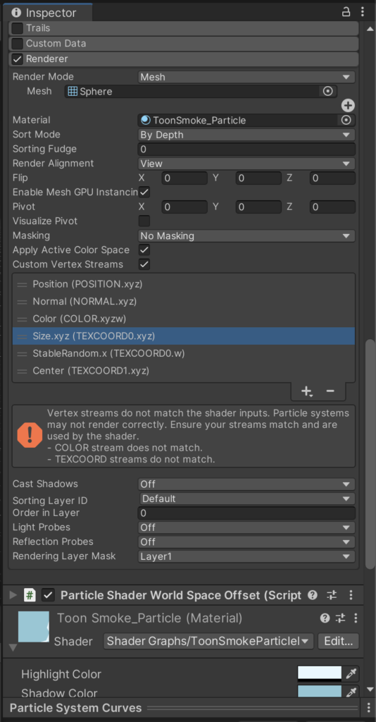
The Unity team, with their latest release of Unity 2021.2, has introduced a slew of improvements to the (relatively new) 2D Rendering Pipeline. If you aren’t familiar yet with the 2D Renderer, it comes with a particularly compelling feature, 2D Lighting, which we can use to performantly light a 2D scene with many simultaneous lights at a time.

The recently-released Tails of Iron by developers Odd Bug Studio uses the 2D Lighting system in Unity.

New in Unity 2021.2 is the introduction of Custom 2D lighting, via the Sprite Custom Lit shader for Shader Graph. It behaves similarly to the normal 2D Lit shader (which lights sprites with realistic, physical calculations), however, it allows us to directly control how the lighting of the scene is applied to our sprites and textures. This opens up quite a few possibilities for us to change the look of our games via the lighting system.

A Custom 2D Toon Shader using multiple Light Textures, used to apply HDR color information to a sprite.

With this tutorial, we’ll introduce a scaled-down version of the above shader, that hopefully ends up being a helpful base to stack on more advanced lighting effects later down the line. This tutorial will assume at least some familiarity with Unity’s Shader Graph, as well as with basic shader concepts.

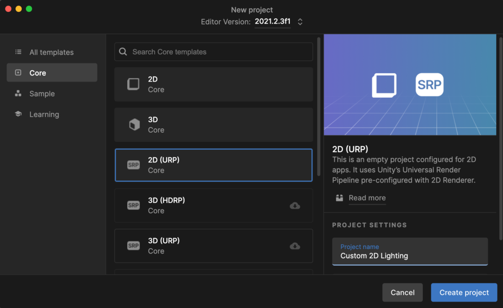
Let’s start by creating a new project in 2021.2, using 2D (URP) as the Project Template. This will set up a new project with an already-configured URP Renderer and 2D Rendering Pipeline for us.

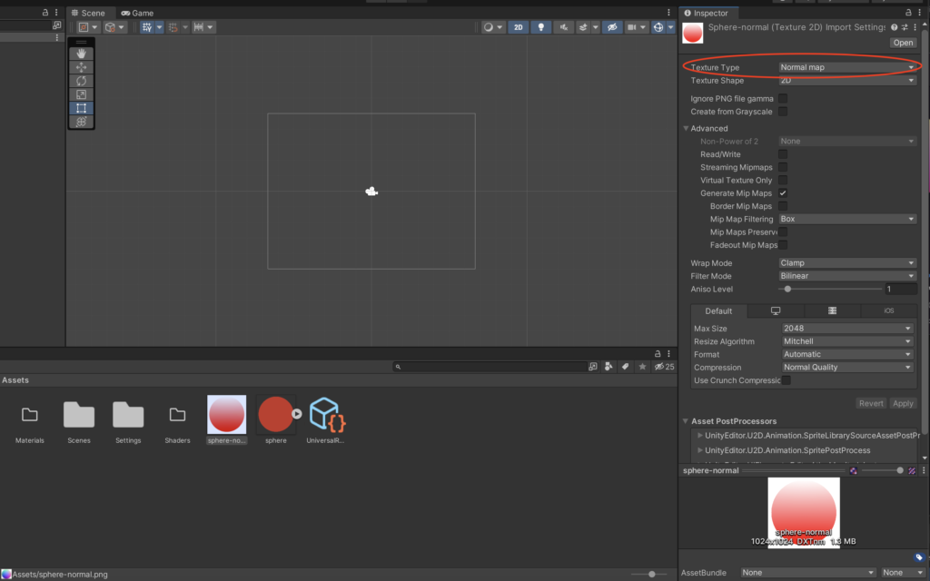
After hitting “Create project”, download the archive below and add sphere.png and sphere-normal.png to the project. This will give us a plain circle sprite, and a corresponding Normal map that’s been generated from a sphere, that’ll let us map 3D information onto the main circle inside of our shaders. This tutorial will assume familiarity with Normal maps, but if they’re a concept that you need to brush up on, here is a decent series that explains them at a fairly informal level.

Note: the tutorial above is for geometry in 3D space, however, it is still applicable for us in 2D as well, as all of the sprites we use are simply 3D quads that have been arranged onto a 2D plane. From a geometry standpoint, there are practically no differences in this respect between 3D Unity scenes and “2D” Unity scenes.

Once the files are in the project, select sphere-normal.png and, under its import settings, set Texture Type to Normal map. This lets Unity know that the texture contains Normal-space information.

Set Texture Type to Normal map in the inspector settings for our sphere’s Normal.

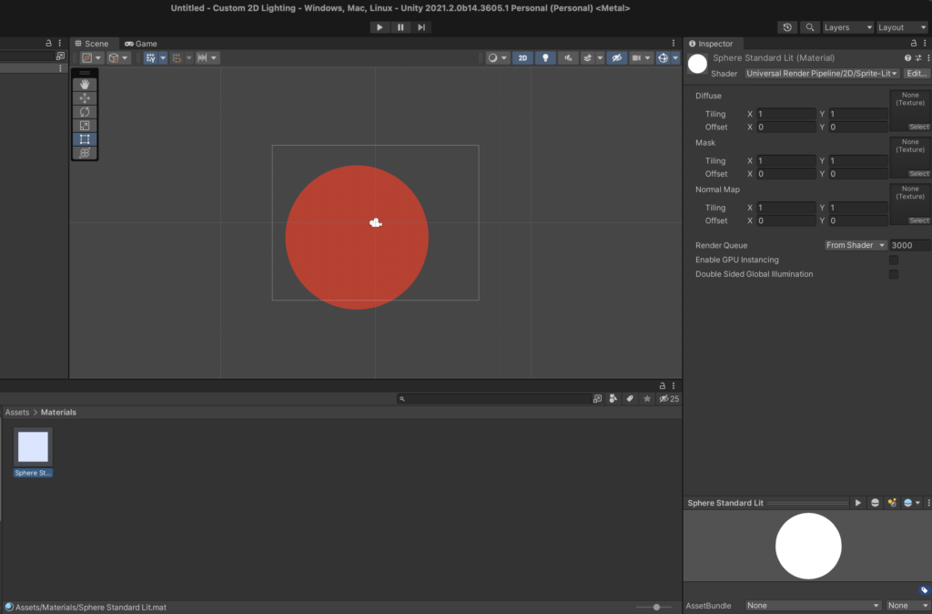
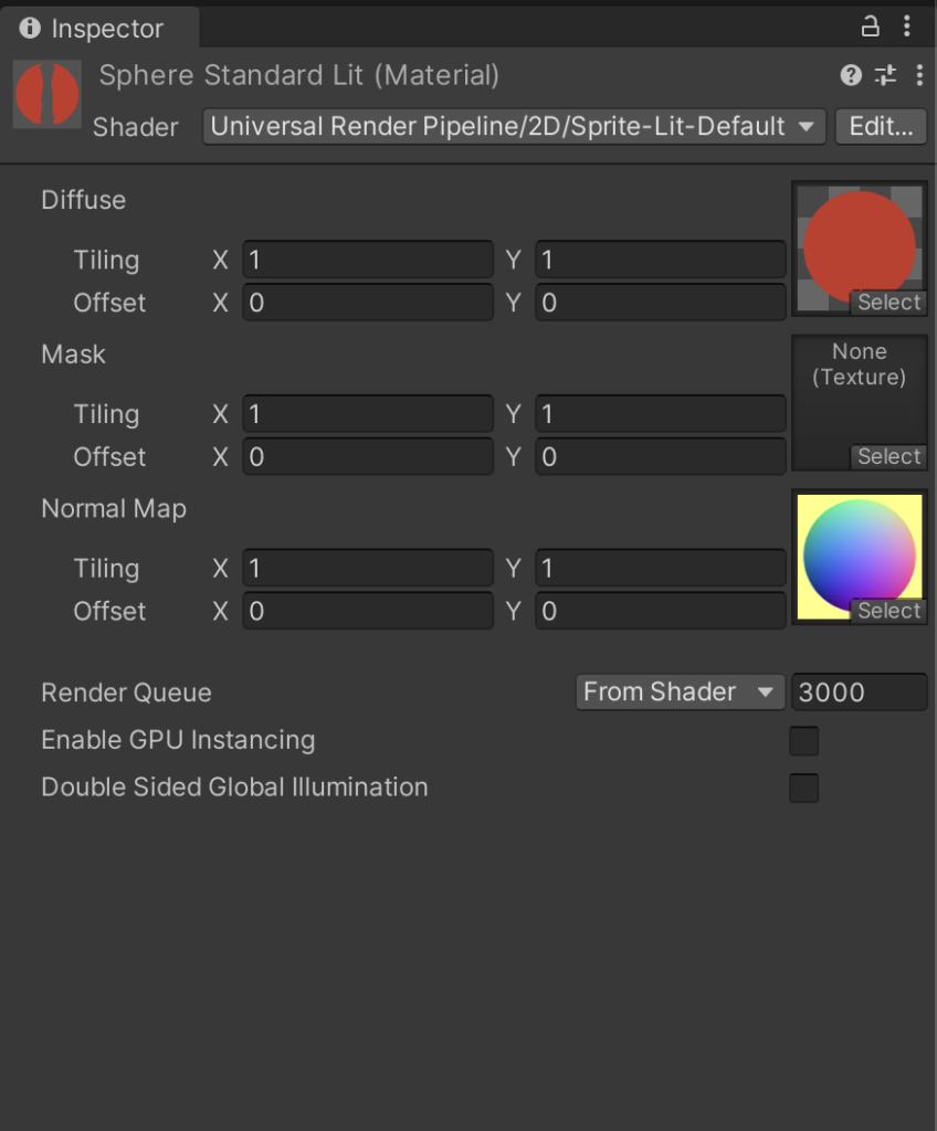
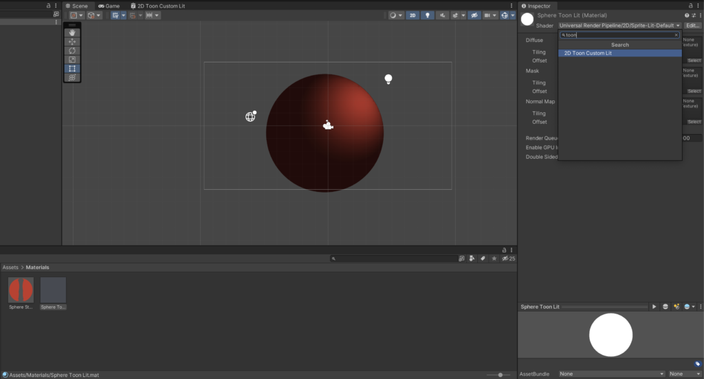
To illustrate how lighting works with the default lit shader, let’s create a new material with the default Sprite Lit 2D shader. Additionally, assign the Normal Map texture in the material to sphere-normal.png. We’ll use this material to sanity-check that basic lighting is working in our scene as expected.

Right Click → Create → Material, then set the Shader property in the inspector to Universal Render Pipeline/2D/Sprite-Lit
Make sure to assign the Normal Map to the material so it can feed that texture to the standard lit shader.

Our next step after setting up this material is to open up the default scene that’s included in the default 2D Template. We’ll do the rest of the tutorial within this scene.

The 2D Template we’re using has an already-set-up scene for us at /Settings/Lit 2D Scene. It includes a Camera and a 2D Global light.

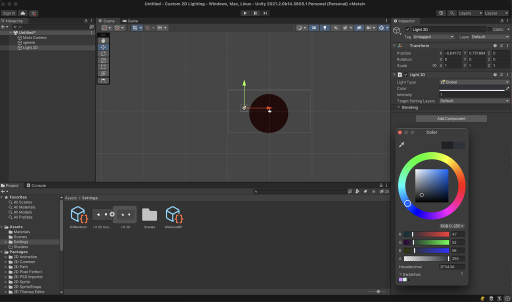
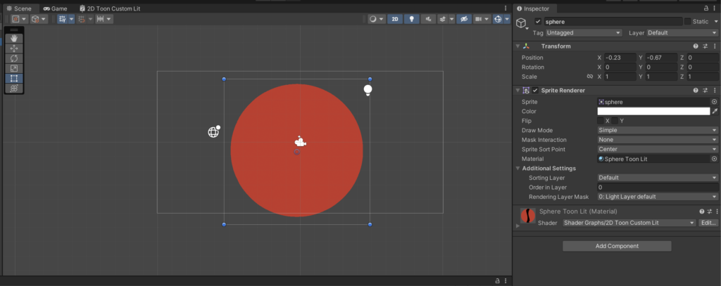
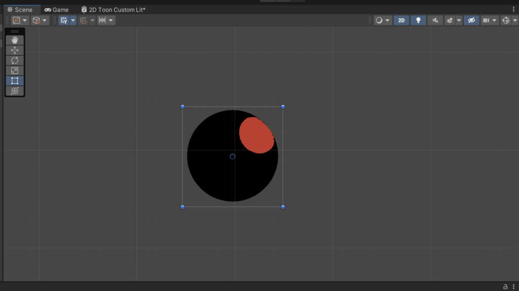
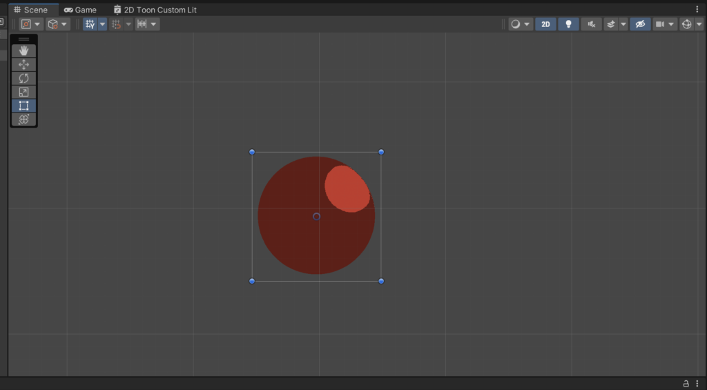
Place the sphere.png sprite into the scene, assign our material to it, and then give the Global Light in the scene a cool, dark color. The sphere should then darken.

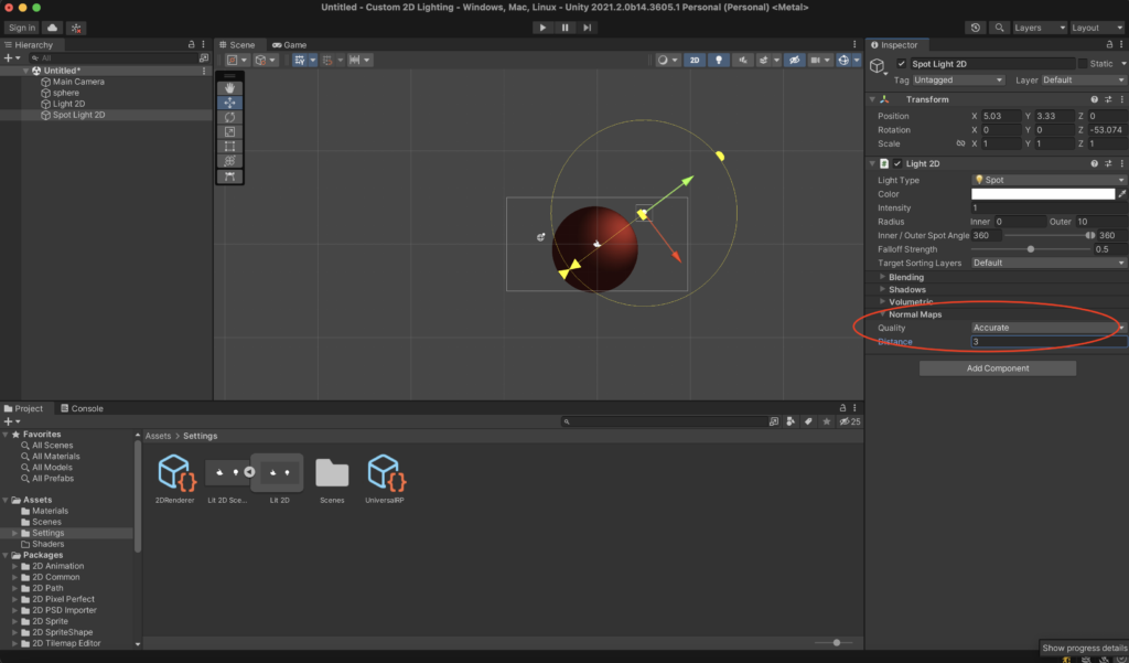
We should be able to light the sphere now via 2D Lighting. Place a 2D Spot Light into the scene and then position it near the sphere. At first, the light should bounce onto the sphere as if it were a flat circle. This is because we need to change the Normal Maps setting of the light to Accurate. Once we do that, the light will respect the Normal information on the sphere’s material, and will light it as if it were a “3D” object.

GameObject → Light → Spotlight 2D. Set the Normal Maps setting to either Fast or Accurate or else the 2D Renderer will light the sphere as if it were a flat object.

We’re fully set up at this point, and can now start deviating from the default Sprite Lit shader by introducing a new, custom shader into our project. Our goal will be to switch from the default shader’s realistic shading to a more stylized, two-tone Toon shader. The hope here is to build a more fitting aesthetic for certain styles of games.

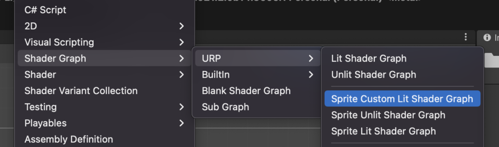
Create a new Sprite Custom Lit Shader Graph (we’ll name it 2D Toon Custom Lit in our project), and then open it to put us into the graph editor.

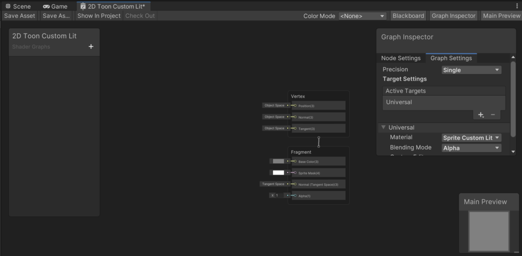
If you’ve used the Sprite Lit Shader Graph in the past, you’ll notice that the Custom Lit graph looks almost identical. The only immediately observable difference from the interface is the addition of the Normal (Tangent Space) output to the Fragment Shader portion.

The addition of the Normal (Tangent Space) output lets the Custom Lit Shader Graph feed in lighting information to the Fragment stage of the shader. We’ll discuss exactly how this works after setting up a few initial things.

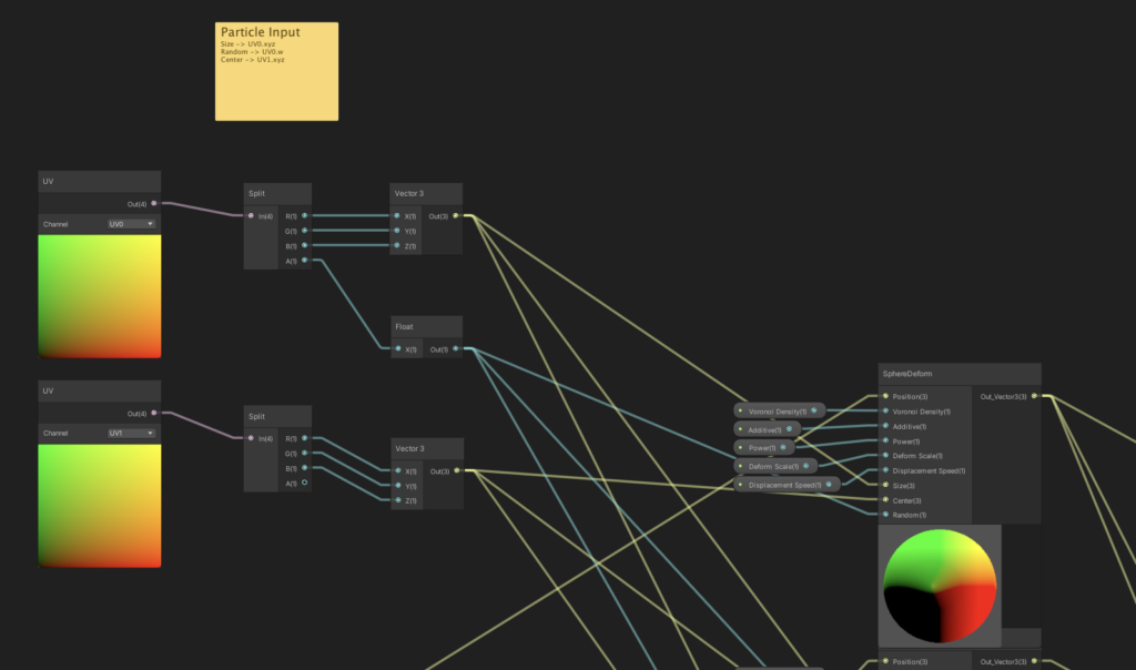
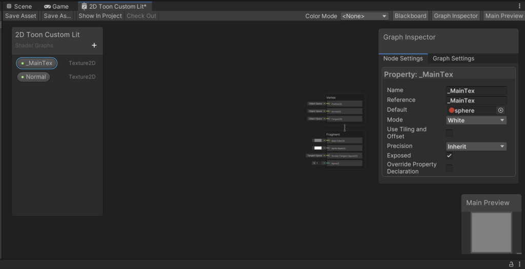
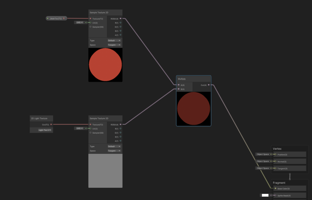
First, let’s create a few inputs for our shader. On the left, inside of the Blackboard pane, create a _MainTex and a Normal Texture2D input. We’ll use these to feed in our sprite and its corresponding normal, in the same manner that we did with the Sprite Lit material.

Blackboard → + Button → Texture 2D

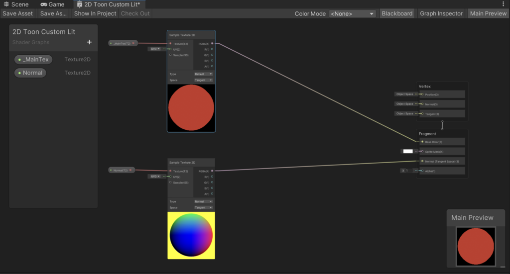
Now let’s connect up our inputs. Create two Sample Texture 2D Nodes, input _MainTex and Normal into their Texture slots, and then feed the _MainTex texture into the BaseColor slot of the Fragment output, and the Normal texture into the Normal (Tangent Space) output. As the Normal output implies, make sure that the Sample Texture 2D node for the Normal texture is set to Type → Normal and Space → Tangent. Hit “Save Asset” in the top left.

We can test the shader in our scene now so we can see how it differs from the Standard Lit shader.

Create a new material, give it our 2D Toon Custom Lit shader, set the material’s _MainTex and Normal textures, and then assign the new material to our sphere sprite.

You’ll notice immediately that our new material is “unlit”. This is expected and is the main difference between the Custom Lit shading path and the Standard path. In the custom shader, we’ll have to apply the lighting ourselves, whereas the Standard Lit shader applies lighting automatically as a separate phase after the main shader runs.

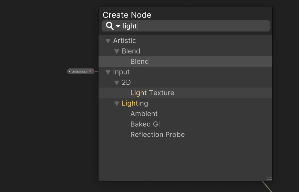
Thankfully, this isn’t too hard to do. The Custom Lit shader exposes a new Node for us, called Light Texture. This node contains the scene’s intermediary lighting information, in the form of a screen-space texture. Conveniently, it respects the Normal information that we’ve outputted to the Normal (Tangent Space) slot, so all of the standard lighting calculations are still handled by the renderer for us.

Let’s add a Light Texture node to our Shader Graph.

Right Click → Create Node, then search for Light Texture.

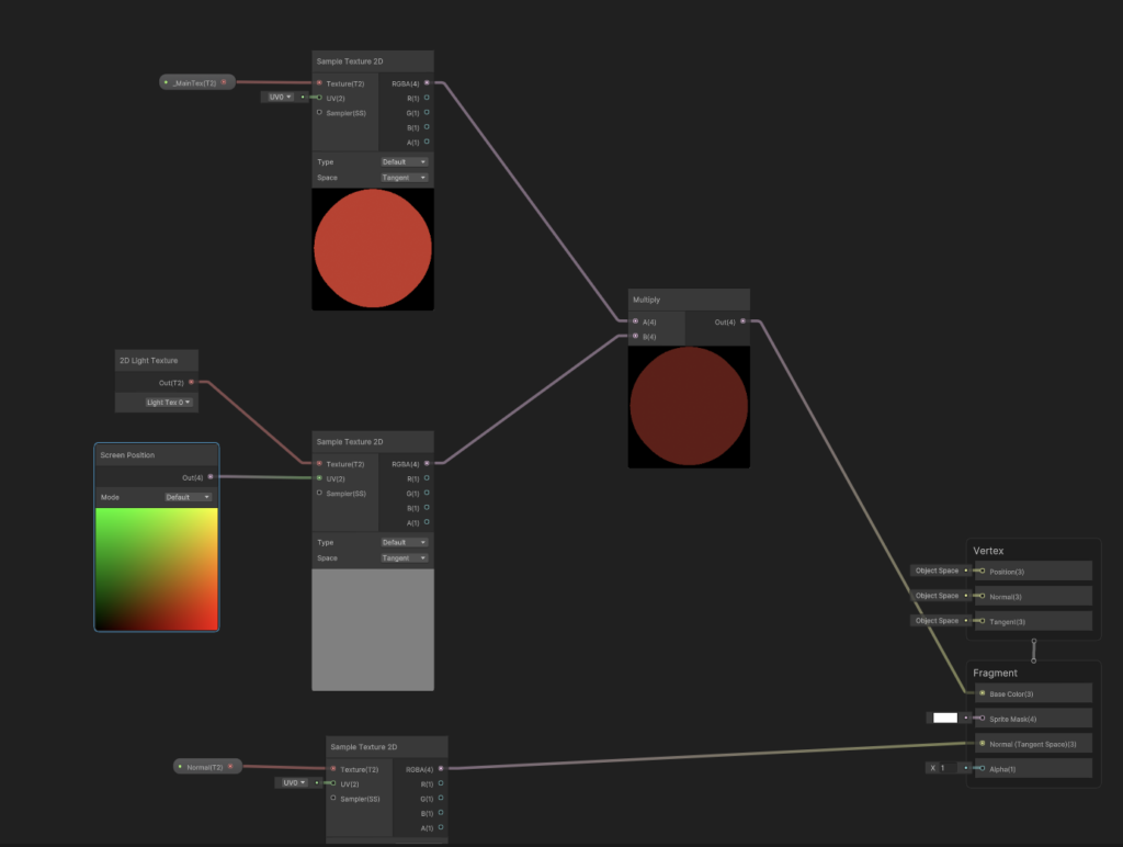
Create another Sample Texture 2D Node, feed our 2D Light Texture into it, and then we’ll multiply the light texture by the Main Texture of our sprite. Feed this into the Base Color output, and then hit Save Asset so we can check out what happens to our scene.

You’ll notice a strange result. There is some lighting info projected onto the sphere, but it’s distorted and centered onto only a small part of the sphere.

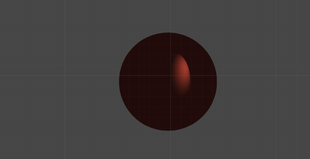
The reason for this is that the 2D Light Texture that we’re sampling contains the lighting texture for the whole screen, and not just the object that we’re applying the shader to. We’re actually projecting the entire screen onto the sphere in our current implementation, but thankfully this is an easy fix.

Let’s go back to the graph so we can feed in screen-space UV coordinates to our Light Texture’s Sample Texture 2D node. Screen Position is a handy node that converts the object’s current UV coordinates into screen-space coordinates, letting us sample only from the portion of the light texture that the object is currently positioned in.

Right Click → Create Node → Screen Position, then feed the output to the UV of our Light Texture’s Sample Texture 2D

Let’s check out our sphere now.

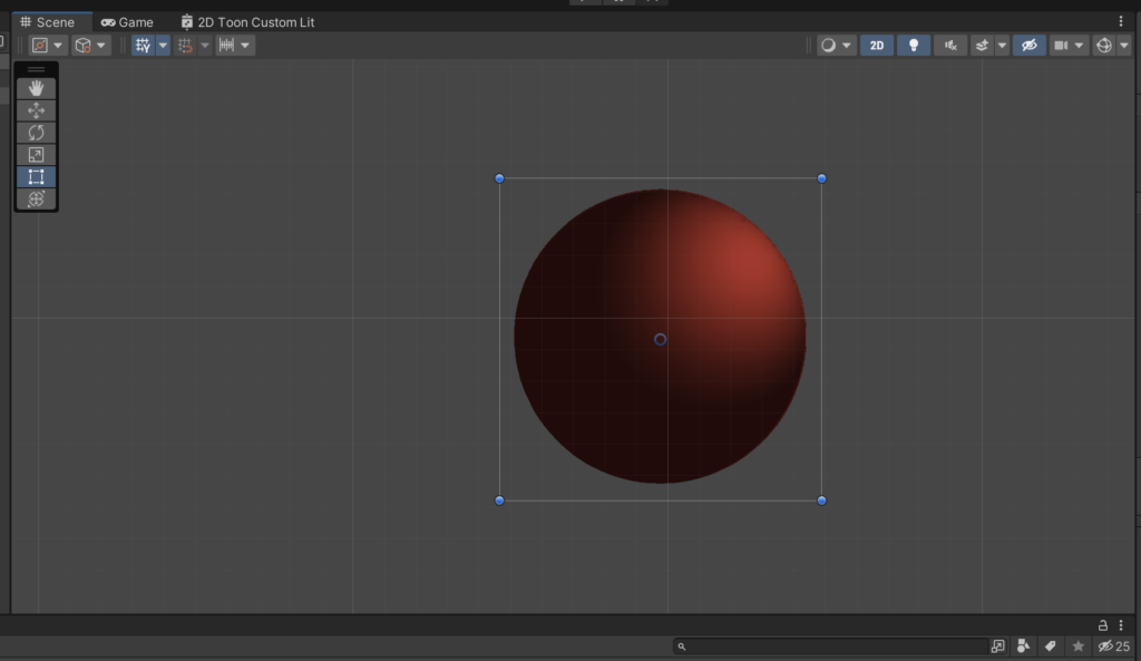
Looking good! We’ve successfully replicated (most) of the Standard Lit shader with our Custom Lit shader. From here, we can start applying some techniques to give us a more stylized lighting projection, as opposed to the simple multiplying of the light texture that we’re doing currently.

The main idea behind a “Toon” shader is to split the light into two “tones” (a light and a dark tone), and then, instead of lighting an object with a smooth gradient between the two tones as we’re doing above, the toon shader will apply the light using a sharp, immediate step between the tones. This is what gives lighting a more cell-shaded look.

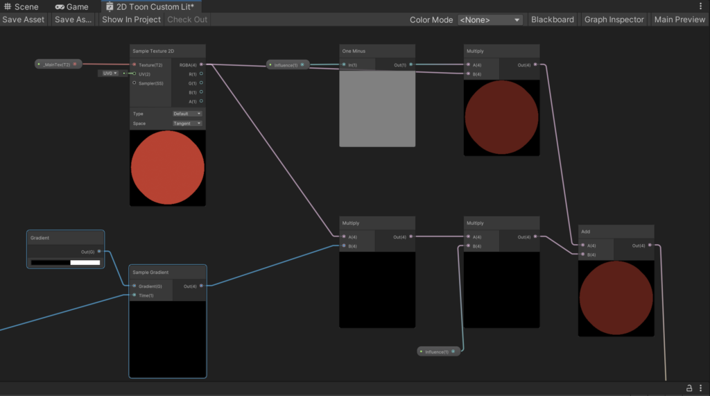
We’ll introduce two more nodes to the graph. The Gradient node, and the Sample Gradient node. Sample Gradient takes two inputs: the first, a Gradient of color information, and the second, a Time value from [0, 1] that maps into the gradient (a value of 0 will take the color at the left-most side of the gradient, and a value of 1 will take the right-most value. Values in-between will select a corresponding intermediary value.)

By giving the Gradient node a Fixed gradient with only two colors (black, and white), we can achieve our “two”-tone look.

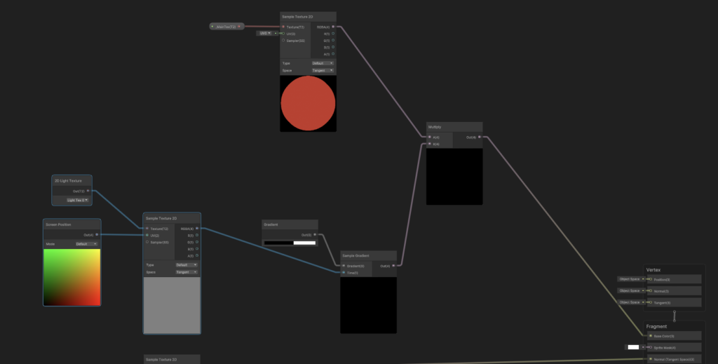
Select the color bar on the Gradient Node, switch the mode from Blend to Fixed, and then give the gradient a black value on the left, and a white value on the right, cut roughly down the middle.

Multiply the output by our Main texture, hit Save Asset, and then check the result in our scene.

We’ll notice that the sphere is being lit by two tones, and in a way that we can expect from our operations in the graph. Values more towards the light (and closer to a value of 1), are being multiplied by the right side of the gradient, which is a value of 1. Thus, they’re left unchanged from the original texture.

Likewise, values further away from the light (and closer to a value of 0) are being multiplied by the left side of the gradient, or by the value 0, and become completely black.

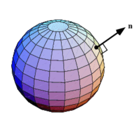
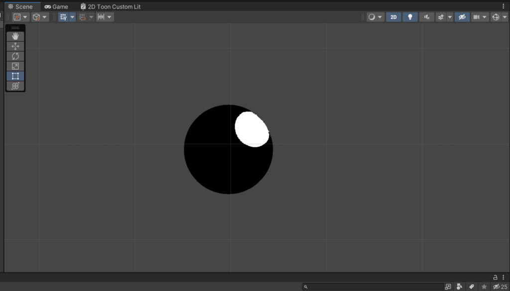
Here’s an illustration of the Gradient map, sans any multiplying to the base color of the main texture.

Our unapplied two-tone lighting information. We project this onto our main sprite to give us our stylized look.

Our goal now is going to be to reduce the contrast of this gradient map, giving us a less intense transition between the regions in shadow and the regions in light. There are a few ways to do this:

  • We could control the colors of our Sample Gradient directly, giving a lighter color to the shadow.
  • Or, we could introduce a “Shadow Strength” parameter that lessens the strength of the black portion of the gradient during our multiplication step.
  • More complicated yet, we could introduce a new parameter, Influence, and then using a standard Mix formula to apply the black and white lighting information to the texture’s base color according to how strong we want the influence of the black and white gradient to be.

All of these are perfectly workable solutions — for the sake of introducing a new concept, we’ll go with the Mix option, even if it’s slightly more complicated. If anything, it’s a new formula that you might find useful for other applications.

Blackboard → + Button → Float. It’s helpful to give this a default value in the Graph Inspector (here we used 0.5), so it can be visualized directly through the node viewers in the Graph.

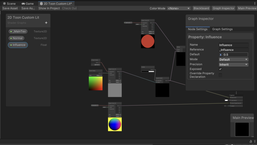
The generic formula for mixing two colors based on an Influence parameter is as follows: ((1 – Influence) * A) + (A * B * Influence). Let’s set this up in the Graph, as shown below.

Finally, connect the result to the Base Color output, hit Save Asset (for the last time), and then check out the sphere.

Looking pretty good! Definitely a different style from the Standard Lit shader, and we can be pretty happy with the result. It’s important to note that this approach does come with some drawbacks, however:

  • We lose color information from the light (because we’re only applying a black and white gradient to the sphere). There are techniques to re-introduce color information, like extracting Hue from the light texture. These work to varying degrees of success.
  • This works best if every lit object in a scene has a Normal map texture, which can increase our workload when creating assets
  • We do get some aliasing between the two tones. There are techniques to fix this, but they’re beyond the scope of this tutorial

That being said, this base shader is still quite powerful on its own.

I’m attaching the Graph below, please feel free to use it for your own projects if you think you could make use of it!


If you'd like to receive notifications whenever this blog has new posts, you can subscribe below. I promise I'll never spam you.
Loading


Building a Toon Smoke Particle Shader in Shader Graph

Two-toned, cartoon-styled artwork and graphical shaders are exceptionally popular lately (see the game Zelda: Breath of the Wild, the similarly inspired Genshin Impact, etc.), so I wanted to make a tutorial that did a bit of a deep-dive into that world, creating a Smoke VFX Shader from scratch.

The information in here is going to be more on the intermediate side. I’ll try my best to explain graphical concepts that aren’t very intuitive (or, more likely, I’ll link away to other resources that can do a much better job of explaining than I can). More importantly, I’m hoping to expose a few concepts that, while being standard in the graphics world, can be hard to come across and learn about if you’re a beginner.

I’ve also derived a fair bit of this shader from other tutorials — I’ll call out those resources within the article whenever we get to a part that cribs from one.

Let’s begin!

Part 1 – Toon Shading a Sphere

Our first goal is going to be adding a two-tone shading to a sphere. For our purposes, we’re not interested in dynamic lighting and will instead control our lighting direction based on a parameter. We’ll also set the base color of each tone directly from the material, so we can stylize the sphere exactly to our liking.

Let’s start by setting up a new Universal Rendering Pipeline project, and then we’ll create an Unlit Shader Graph.

Right Click — Create → Shader → Universal Render Pipeline → Unlit Shader Graph

We’re just focused on coloring for now, so we’ll be working on the lower portion of the Shader Graph (the fragment shader portion). Our goals here are as follows:

  • Input a highlight color, a shadow color, and a light direction into the shader.
  • Color the sections facing the “light” with the highlight color, and color the sections angled away from the “light” with the shadow color.

We can do the first part pretty quickly by adding three inputs to the shader, like so:

Blackboard → + Button → Color/Vector3

Figuring out which portions of the sphere are facing the light is relatively straightforward, too. We’ll take the dot product of the light direction vector and of the current Normal, which will then spit back a value from 1 to -1 (we get a nice [-1, 1] range only if both vectors are unit vectors, otherwise the range depends on the magnitude of each vector). Essentially, the dot product tells us how “aligned” the two angles are. We get 1 if the normal is perfectly facing light, 0 if it’s at a 90º angle, and -1 if it is facing entirely away from the light. We’ll also introduce an extra “Shadow Attenuation” parameter to give us a little more control over how much of the sphere is in highlight vs. shadow.

This is a common way to calculate lighting on an object — common enough that it’s known colloquially as NdotL. We’ll clamp this output from 0 to 1, so that way all negative values (or, values facing away from the light) are completely shadowed.

The “Saturate” node will clamp our Dot Product to the range [0, 1]. The “Normalize” node takes our light direction and converts it to a unit vector. The Normal Vector (the top-left-most node) is already “Normalized”, so we don’t need to do anything additional to it.

From here, we’ll posterize the dot product into two discrete values, and then use that value to lerp between our two colors. We select the shadow color if we’re closer to 0, and the highlight color if we’re closer to 1.

Pipe this into the ‘Base Color’ output of our Fragment shader, and then we should be pretty solid. Let’s check this in the scene view by creating a material and then assigning it to a sphere.

Looking pretty decent! This is a very basic way to two-tone shade a mesh, but it’s good enough for our purposes. We can eventually add more depth to this by introducing features such as multiple posterization steps, specular highlights, dynamic lighting, etc., but these are definitely topics for another tutorial.

Part 2 – Deforming the Sphere

Our next goal is to add some amount of random deformation to the sphere, to break things up and make the sphere look more “smoke-like”. There are a bunch of techniques on how to do this, but the majority of them boil down to a relatively simple concept — take the normal vector of each vertex, and then apply some kind of +/- offset in the direction of that normal to the position of the vertex on the mesh. This “pulls” and “pushes” the vertices of our sphere.

For this portion, we’re working in the upper part of the Shader Graph (the vertex shader portion). Our goals are to:

  • Take the position and normal of each vertex
  • In the direction of each normal, calculate a +/- offset
  • Add that offset to the associated vertex position

Smooth random noise generators output a value from 0 to 1 based on the UV index we input. In a Voronoi generator, indexes close to each other will be similar in value.

We don’t want to apply a completely random offset to each vertex, else we’ll risk the sphere looking spikey and very unsmoke-like. Instead, a common technique is to pipe the position of each vertex into a smooth noise generator, so that positions that are closer to each other have a smaller change in offset. There are many ways to do this: for this tutorial, we’ll use a cool approach with Voronoi Noise that I came across via this video, however using a simple gradient noise works almost just as well.

Let’s recreate the graph from that video. There are a few additional steps of math that let us parameterize how the sphere deforms, but I won’t go into the fine details around that in this tutorial.

Make sure the “Position” input is set to “Object” space.

Take our resulting output, multiply it by a “Scale” input to give us a bit of further control, and then multiply it by our vertex’s Normal Vector.

And then, to have this do anything, we’ll add our output at the end to the original position of the node, and then pipe that to the “Vertex” output of our shader.

And then if we check our Sphere in the scene view, we’ll see that it’s starting to deform a bit. Unfortunately, we still have a lot to do! However the name of the game here is small incremental progress.

We want the smoke to animate, of course, so we’ll also pipe in an offset to the random noise input based on the current clock time. We’ll also multiply the clock time by a constant to give us some control over how fast or how slow the offset changes.

We should be good now. Checking this out in the scene view, we’ll see the deform animation in play.

One question you might be asking is — why is the center part of the sphere being shaded as if it were a near-perfect circle? When in theory, the deformation should be breaking up that portion, giving us some additional definition and shadow in the body of the sphere.

The answer boils down to the sphere’s current Normal Vectors. In our shader right now, we’re displacing each of our vertices without modifying their Normal Vectors to match. And because our toon shading is entirely controlled by the Normal information of each vertex, we end up shading each face as if it were positioned on a perfectly-round sphere.

We’ll go over the solution to this problem in Part 3. Unfortunately, things start to get a little complicated from here, but it’s nothing that we can’t manage.

Part 3 – Normal Correction

A big thanks to @GameDevBill for writing a great tutorial on this subject. A large portion of this following section will use concepts and graphs from that write-up.

I’d recommend reading the above tutorial if you have the time — Bill does more in-depth (and certainly much better) explanation of what’s going on here than what I’m capable of. I’ll do a brief summary below, and then we’ll work on modifying our Shader Graph.

Each “color” of the sphere represents a Normal direction.

Adjacent is an image of an unmodified sphere and its colored normal faces. The most important thing to understand is that the normal “colors” here are encoded as separate data alongside the rest of the sphere’s mesh (they are not calculated on the fly based on the current direction of the face). Given that, you can imagine that if we took each of the sphere’s vertexes and arbitrarily displaced them, the “color” of each face would remain the same, while each face’s physical location and orientation would change.

Our goal then is to find a way to re-calcuate each vertex’s normal direction to better match the physical direction it becomes oriented in after deformation. There are a few ways to do this (a common theme here in graphics), but we’re going to take a “good-enough” approach that is relatively easy to think about conceptually.

Given a point on our mesh, we’re able to calculate a normal direction for it by taking the cross product of two additional points on the same plane as that point.

The cross product gives us the perpendicular direction of two vectors in 3D space.

So, for each vertex on our sphere, we’ll find two additional points that are approximately very close to it, and then deform those points in the same way that we’ve deformed our original vertex. We’ll then run a cross product on our new points to get an approximate normal vector.

The graph for grabbing additional adjacent points is unfortunately a little complicated. I’ll include the sub-graph below for you to include in your project.

Now is also a good time to split the parts we’ve already written into separate sub-graphs. We’ll want to re-use the deform logic to be able to find our two adjacent points, so this is a useful step for us beyond the primary benefit of keeping things readable.

Highlight → Right Click / Convert To → Sub-graph

Insert the downloaded ‘Neighbors’ sub-graph into our main graph, and pipe the Position input into it. Take the resulting two points and apply our deform sub-graph to them as well.

This triples the cost of our shader, but the trade-off is worth it in most cases.

Finally, we’ll calculate two resultant vectors, normalize them, and then take the cross product. We then feed that into the “Normal” output of the shader.

Check out our sphere now in the scene view. It’s looking much better!

Our last step in this tutorial is to feed this material into a particle system, for dynamic-looking smoke. Unfortunately, our work is not done yet, as we’ll need a few adjustments to our shader to have it work on a per-particle basis.

Part 4 – Working with the Particle System

If we set up a Particle System right now, and applied our material to it, we’d end up with something that looked like this.

Some observations:

  • The deformation is blowing up, causing each offset to blow past our clamped bounds (and thus giving each particle a perfectly spherical shape)
  • As each particle moves, its deformation speed gets much faster (slightly hard to notice in this video)

To understand why each of these issues occur, we need to understand a little more about what happens to meshes when they’re fed into a Particle System.

For (very important) performance reasons, Unity batches each mesh in a Particle System into one combined mesh. There is a lot of technical detail in that process that I’m going to hand-wave away, but it has some practical implications that affect us. Particularly, each vertex within the Particle System gets transposed to World Space — within a particle system, we have no built-in way of accessing the object-local positions of a sphere’s vertices.

This means that, for each vertex that we process in our current shader:

  • The offset we calculate will be the same unit magnitude for every sphere, no matter the sphere’s current size (“size” isn’t a concept in our shader currently — our only input is “position”)
  • As each particle in the system moves, their vertices’s positions will change as well (as each vertex is translated into World Space)

Fortunately, Unity provides a facility named Particle Vertex Streams that allows us to input particle-specific data into our shader. We can solve our above problems by a) taking the “Size” parameter of each particle as input, and then normalizing our deformation offsets based off of that, and then b) transforming each vertex position into local space, using the particle’s “Center” parameter (alongside an additional World Position parameter that we’ll add to the overall material, via Material Property Block).

Lastly, we’ll input a random per-particle value and use it to offset our deformation. This will give each particle in the system some additional variation.

Enable the ‘Custom Vertex Streams” checkbox, remove the UV stream (we aren’t using it, so it’s just taking up extra space), and then add the Size, StableRandom, and Center vertex streams. Next to each vertex stream is the channel that it’s input to the shader as. For example, Size is input via the UV0 channel, via the x, y, and z segments of the vector.

We’ll hook up the inputs inside of our graph now. Add “Size”, “Center”, and “Random” inputs into our deform sub-graph as well, and then make sure all of the wires are crossed correctly.

Additionally, we need to input the “World Position” of our Particle System GameObject into this shader. Our general strategy is to, for each particle, find the offset between the particle’s center and our system’s center, and then we’ll apply that offset to each of our particle’s vertices. This keeps each vertex to a local coordinate space, regardless of how it moves within the overall batched Particle System. Doing this is key to prevent the particle from deforming in unwanted ways as it moves through the world.

using UnityEngine;

[ExecuteInEditMode]
[RequireComponent(typeof(Renderer))]
public class ParticleShaderWorldSpaceOffset : MonoBehaviour
{
    Renderer _renderer;

    static readonly int WorldPos = Shader.PropertyToID("WorldPos");

    MaterialPropertyBlock _propBlock;
    
    void Awake() {
        _renderer = GetComponent<Renderer>();
        _propBlock = new MaterialPropertyBlock();
    }

    void Update() {
        _renderer.GetPropertyBlock(_propBlock);
        Vector3 existingWorldPos = _propBlock.GetVector(WorldPos);
        if (existingWorldPos != transform.position) {
            _propBlock.SetVector(WorldPos, transform.position);
            _renderer.SetPropertyBlock(_propBlock);
        }
    }
}

Add a “WorldPos” property to our shader (and to our deform sub-graph), and attach the following script to our Particle System. This will, every frame, update our shader with the World Position of our system, via Material Property Block.

In the deform sub-graph, our first step is to transform our input position into a local coordinate, and then to divide that position by our “size” input. This will give us a local, normalized position that we can feed into our noise.

Feed this output into our two Tiling and Offset nodes.

From there, the only other step is to, after calculating our offset, multiplying it back by our “Size” parameter, so that we’re offsetting by an amount that’s in-line with how big our sphere is.

Without this step, our offsets will be too large for small particle sizes, as seen in the video at the start of this section.

Last step (and I mean it this time!), add a random range to our time offset, introducing a small amount of variability between the particles.

Let’s save our graph and check things out!

Smoke!

I think the smoke is looking pretty decent at this point. Things definitely converged a little late with our approach here, but we’ll finally shelve this one and call it done.

I’m attaching the Shader Graph for this smoke effect below. I hope you find it useful. Good luck!


If you'd like to receive notifications whenever this blog has new posts, you can subscribe below. I promise I'll never spam you.
Loading
 

Running WordPress Behind SSL and NGINX Reverse Proxy

A common hosting configuration for web applications (like WordPress! which this site unsurprisingly runs on), is to first install the application inside of some kind of isolated environment (e.g. a Virtual Machine or Docker Container), and then use NGINX as a reverse proxy to sort and forward any incoming traffic to its right destination. This is especially handy when dealing with HTTPS-based traffic, as NGINX can terminate each request and then send the raw HTTP traffic to the right application server.

It’s worth nothing that application servers are generally capable of terminating SSL themselves, but they are also generally not as performant at it as NGINX is. Terminating at the reverse proxy level carries a few other benefits, most notably the ability to direct traffic based on the URI of a request (e.g. /en/ vs. /de/, to direct to a different server based on the localization of a site).

The process of configuring this is usually straightforward for most applications. However, in setting up this site, I came across quite a few blog posts around WordPress and SSL that offer pretty bizarre solutions. I’m by no means a WordPress person but please, please do not look for Plugins to hack around a badly set-up WordPress configuration when you’re setting up SSL.

This post is using a WordPress installation via WordPress’s official Docker Repository. The docker-compose.yml file we’re using looks like this.

version: "3.9"
    
services:
  db:
    image: mysql:5.7
    volumes:
      - db_data:/var/lib/mysql
    restart: always
    environment:
      MYSQL_ROOT_PASSWORD: somewordpress
      MYSQL_DATABASE: wordpress
      MYSQL_USER: wordpress
      MYSQL_PASSWORD: wordpress
    
  wordpress:
    depends_on:
      - db
    image: wordpress:latest
    ports:
      - "8000:80"
    restart: always
    environment:
      WORDPRESS_DB_HOST: db:3306
      WORDPRESS_DB_USER: wordpress
      WORDPRESS_DB_PASSWORD: wordpress
      WORDPRESS_DB_NAME: wordpress
volumes:
  db_data: {}

When that’s set up on our server, we’ll bring up WordPress and its backing MySQL Database like so.

docker-compose up -d
Creating network “wordpress_default” with the default driver
Creating volume “wordpress_db_data” with default driver
Creating wordpress_db_1 … done
Creating wordpress_wordpress_1 … done

WordPress should be up at this point. We can access it via port 8000, the port we exposed in the above docker-compose.yml config.

At this point, I’d recommend setting up our NGINX config before proceeding with the installation. That’ll make it so the site is configured with the correct domain name after going through the installation wizard (and not http://10.0.1.11, like in the above example). This can of course be changed later in settings if you do end up doing things in a different order.

A simple NGINX config would look like so.

server {
    listen 80;
    server_name blog.ldev.app;
    rewrite ^(.*) https://$host$1 permanent;
}
server {
    listen 443;
    server_name blog.ldev.app;
    ssl on;
    ssl_certificate /etc/pve/local/nginx/ldev-ssl.pem;
    ssl_certificate_key /etc/pve/local/nginx/ldev-ssl.key;
    proxy_redirect off;
    location / {
        proxy_pass http://10.0.1.11:8000;
    }
}

This listens for incoming traffic on the domain name “blog.ldev.app”, terminates the SSL connection (or, tells the client to redirect to the https:// version of this resource if the initial request came in via http), and forwards the now-decrypted traffic to our WordPress application server at :8000.

Unfortunately, under this configuration, WordPress doesn’t have any way of knowing when incoming requests are sent via HTTPS, and is unable to render HTTPS-based content in response. To see what I mean, if we launch this configuration and navigate to our site, we’ll observe that static content (e.g. the CSS stylesheets) is served using http-relative links. Modern browsers generally prevent the loading of insecure links inside of pages accessed via HTTPS, so things break in a predictable fashion.

What we need to do from here is to pass on a few HTTP headers (via NGINX) to our WordPress application, so WordPress knows that it’s being accessed via HTTPS and can render itself accordingly.

When WordPress processes requests internally, it looks for these headers, as defined in wp-config.php:

if (isset($_SERVER['HTTP_X_FORWARDED_PROTO']) && $_SERVER['HTTP_X_FORWARDED_PROTO'] === 'https') {
  $_SERVER['HTTPS'] = 'on';
} 

Note that, if you are installing WordPress outside of the official Docker repository, you might have to add the above manually to your wp-config.php.

We can fix our situation by adding the following standard fields to our NGINX config.

server {
    listen 443;
    server_name blog.ldev.app;
    ssl on;     ssl_certificate /etc/pve/local/nginx/ldev-ssl.pem;
    ssl_certificate_key /etc/pve/local/nginx/ldev-ssl.key;
    proxy_redirect off;
    location / {
        proxy_set_header        Host $host:$server_port;
        proxy_set_header        X-Real-IP $remote_addr;
        proxy_set_header        X-Forwarded-For $proxy_add_x_forwarded_for;
        proxy_set_header        X-Forwarded-Proto $scheme;
        proxy_pass http://10.0.1.11:8000;
    }
}

Restart the NGINX server, and we should be good to go.

From here, everything should work as expected. WordPress will serve all links as HTTPS, the admin page will function correctly, and we’re ready to start customizing our site.