
Two-toned, cartoon-styled artwork and graphical shaders are exceptionally popular lately (see the game Zelda: Breath of the Wild, the similarly inspired Genshin Impact, etc.), so I wanted to make a tutorial that did a bit of a deep-dive into that world, creating a Smoke VFX Shader from scratch.
The information in here is going to be more on the intermediate side. I’ll try my best to explain graphical concepts that aren’t very intuitive (or, more likely, I’ll link away to other resources that can do a much better job of explaining than I can). More importantly, I’m hoping to expose a few concepts that, while being standard in the graphics world, can be hard to come across and learn about if you’re a beginner.
I’ve also derived a fair bit of this shader from other tutorials — I’ll call out those resources within the article whenever we get to a part that cribs from one.
Let’s begin!
Part 1 – Toon Shading a Sphere
Our first goal is going to be adding a two-tone shading to a sphere. For our purposes, we’re not interested in dynamic lighting and will instead control our lighting direction based on a parameter. We’ll also set the base color of each tone directly from the material, so we can stylize the sphere exactly to our liking.
Let’s start by setting up a new Universal Rendering Pipeline project, and then we’ll create an Unlit Shader Graph.
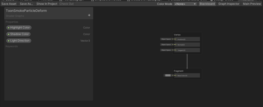
We’re just focused on coloring for now, so we’ll be working on the lower portion of the Shader Graph (the fragment shader portion). Our goals here are as follows:
- Input a highlight color, a shadow color, and a light direction into the shader.
- Color the sections facing the “light” with the highlight color, and color the sections angled away from the “light” with the shadow color.
We can do the first part pretty quickly by adding three inputs to the shader, like so:
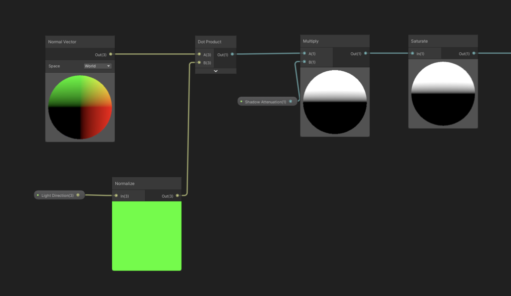
Figuring out which portions of the sphere are facing the light is relatively straightforward, too. We’ll take the dot product of the light direction vector and of the current Normal, which will then spit back a value from 1 to -1 (we get a nice [-1, 1] range only if both vectors are unit vectors, otherwise the range depends on the magnitude of each vector). Essentially, the dot product tells us how “aligned” the two angles are. We get 1 if the normal is perfectly facing light, 0 if it’s at a 90º angle, and -1 if it is facing entirely away from the light. We’ll also introduce an extra “Shadow Attenuation” parameter to give us a little more control over how much of the sphere is in highlight vs. shadow.
This is a common way to calculate lighting on an object — common enough that it’s known colloquially as NdotL. We’ll clamp this output from 0 to 1, so that way all negative values (or, values facing away from the light) are completely shadowed.
From here, we’ll posterize the dot product into two discrete values, and then use that value to lerp between our two colors. We select the shadow color if we’re closer to 0, and the highlight color if we’re closer to 1.
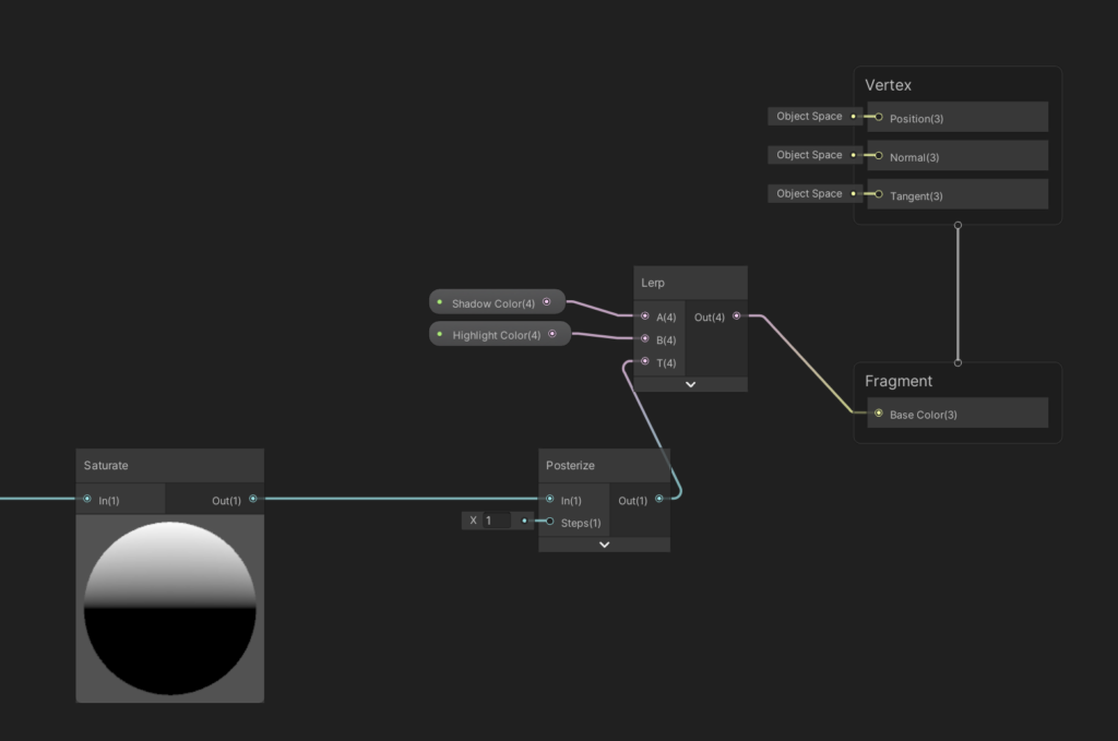
Pipe this into the ‘Base Color’ output of our Fragment shader, and then we should be pretty solid. Let’s check this in the scene view by creating a material and then assigning it to a sphere.
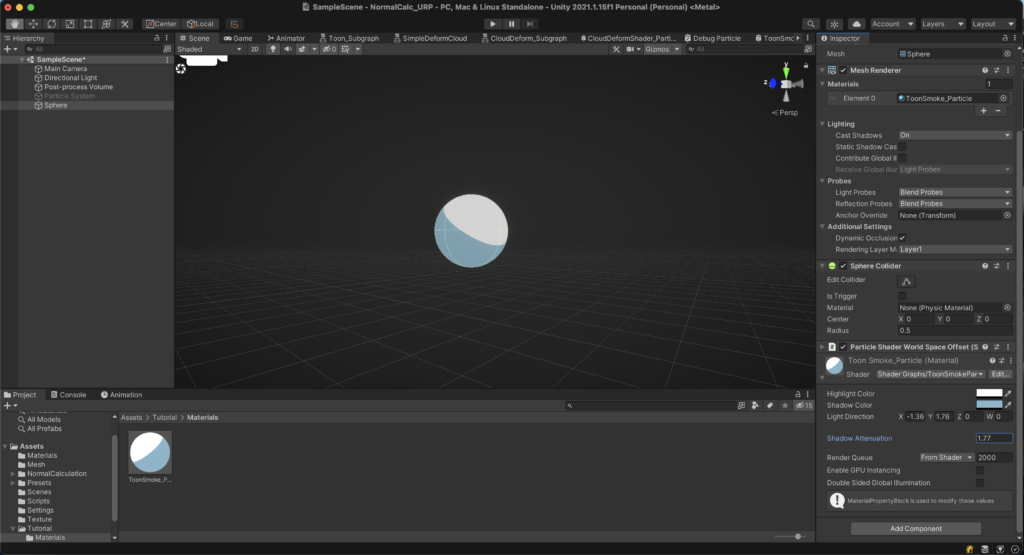
Looking pretty decent! This is a very basic way to two-tone shade a mesh, but it’s good enough for our purposes. We can eventually add more depth to this by introducing features such as multiple posterization steps, specular highlights, dynamic lighting, etc., but these are definitely topics for another tutorial.
Part 2 – Deforming the Sphere
Our next goal is to add some amount of random deformation to the sphere, to break things up and make the sphere look more “smoke-like”. There are a bunch of techniques on how to do this, but the majority of them boil down to a relatively simple concept — take the normal vector of each vertex, and then apply some kind of +/- offset in the direction of that normal to the position of the vertex on the mesh. This “pulls” and “pushes” the vertices of our sphere.
For this portion, we’re working in the upper part of the Shader Graph (the vertex shader portion). Our goals are to:
- Take the position and normal of each vertex
- In the direction of each normal, calculate a +/- offset
- Add that offset to the associated vertex position
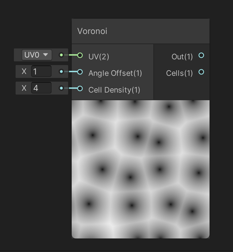
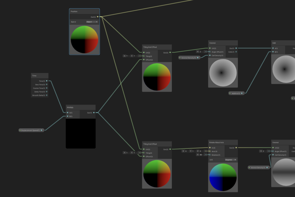
We don’t want to apply a completely random offset to each vertex, else we’ll risk the sphere looking spikey and very unsmoke-like. Instead, a common technique is to pipe the position of each vertex into a smooth noise generator, so that positions that are closer to each other have a smaller change in offset. There are many ways to do this: for this tutorial, we’ll use a cool approach with Voronoi Noise that I came across via this video, however using a simple gradient noise works almost just as well.
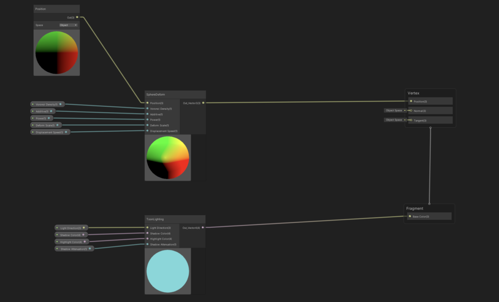
Let’s recreate the graph from that video. There are a few additional steps of math that let us parameterize how the sphere deforms, but I won’t go into the fine details around that in this tutorial.
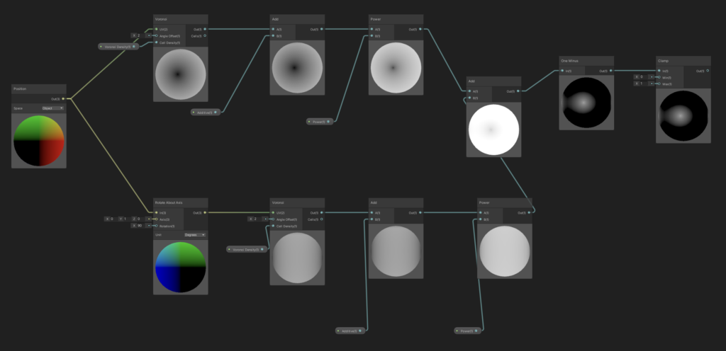
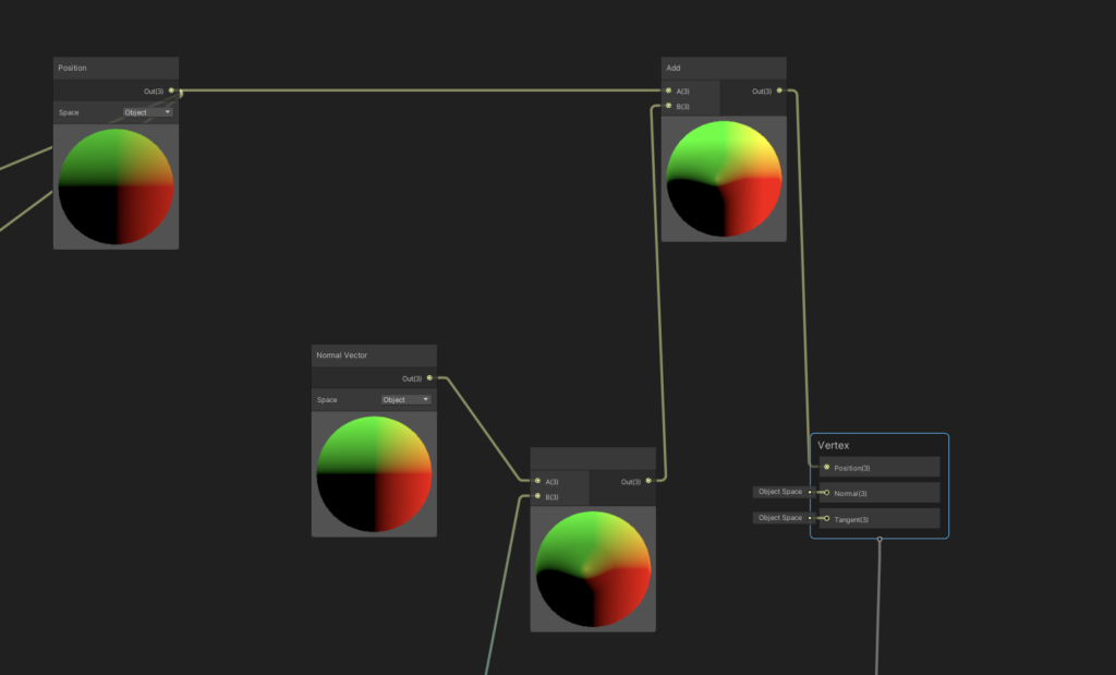
Take our resulting output, multiply it by a “Scale” input to give us a bit of further control, and then multiply it by our vertex’s Normal Vector.
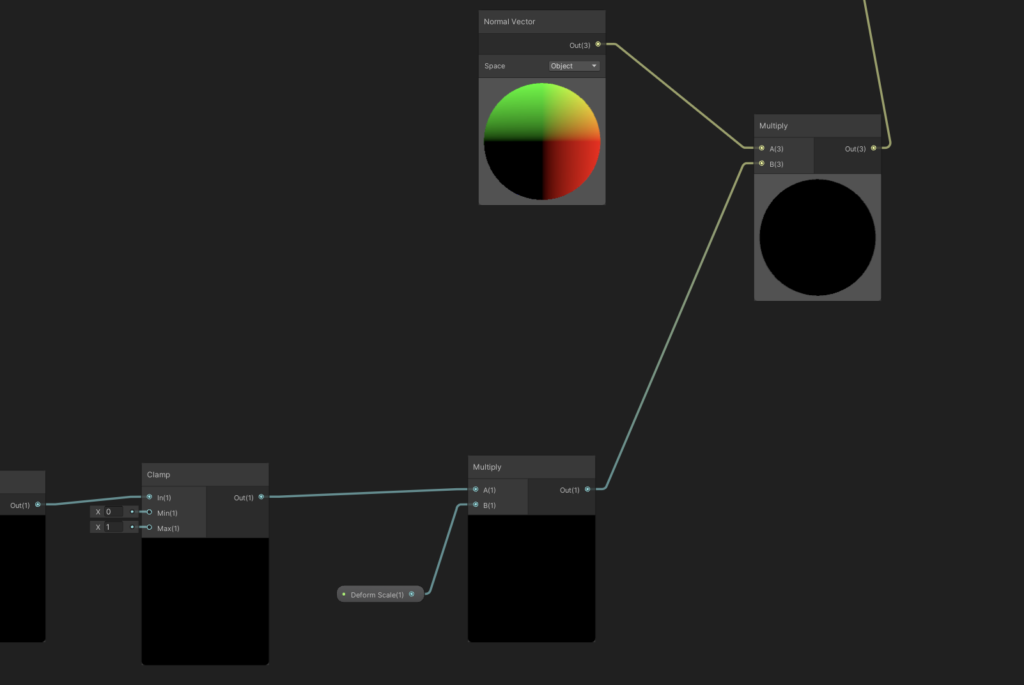
And then, to have this do anything, we’ll add our output at the end to the original position of the node, and then pipe that to the “Vertex” output of our shader.
And then if we check our Sphere in the scene view, we’ll see that it’s starting to deform a bit. Unfortunately, we still have a lot to do! However the name of the game here is small incremental progress.
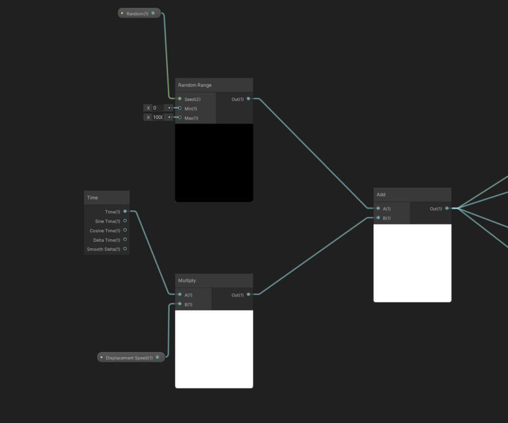
We want the smoke to animate, of course, so we’ll also pipe in an offset to the random noise input based on the current clock time. We’ll also multiply the clock time by a constant to give us some control over how fast or how slow the offset changes.
We should be good now. Checking this out in the scene view, we’ll see the deform animation in play.
One question you might be asking is — why is the center part of the sphere being shaded as if it were a near-perfect circle? When in theory, the deformation should be breaking up that portion, giving us some additional definition and shadow in the body of the sphere.
The answer boils down to the sphere’s current Normal Vectors. In our shader right now, we’re displacing each of our vertices without modifying their Normal Vectors to match. And because our toon shading is entirely controlled by the Normal information of each vertex, we end up shading each face as if it were positioned on a perfectly-round sphere.
We’ll go over the solution to this problem in Part 3. Unfortunately, things start to get a little complicated from here, but it’s nothing that we can’t manage.
Part 3 – Normal Correction
A big thanks to @GameDevBill for writing a great tutorial on this subject. A large portion of this following section will use concepts and graphs from that write-up.
I’d recommend reading the above tutorial if you have the time — Bill does more in-depth (and certainly much better) explanation of what’s going on here than what I’m capable of. I’ll do a brief summary below, and then we’ll work on modifying our Shader Graph.
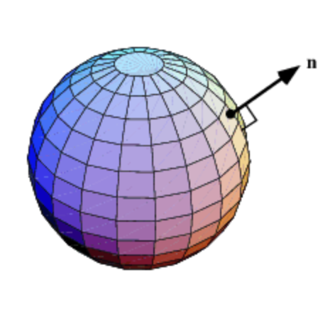
Adjacent is an image of an unmodified sphere and its colored normal faces. The most important thing to understand is that the normal “colors” here are encoded as separate data alongside the rest of the sphere’s mesh (they are not calculated on the fly based on the current direction of the face). Given that, you can imagine that if we took each of the sphere’s vertexes and arbitrarily displaced them, the “color” of each face would remain the same, while each face’s physical location and orientation would change.
Our goal then is to find a way to re-calcuate each vertex’s normal direction to better match the physical direction it becomes oriented in after deformation. There are a few ways to do this (a common theme here in graphics), but we’re going to take a “good-enough” approach that is relatively easy to think about conceptually.
Given a point on our mesh, we’re able to calculate a normal direction for it by taking the cross product of two additional points on the same plane as that point.
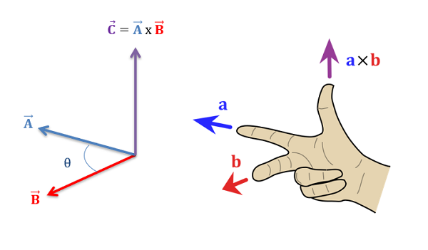
So, for each vertex on our sphere, we’ll find two additional points that are approximately very close to it, and then deform those points in the same way that we’ve deformed our original vertex. We’ll then run a cross product on our new points to get an approximate normal vector.
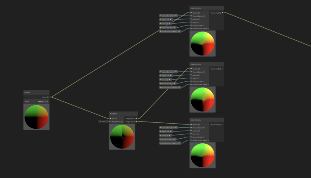
The graph for grabbing additional adjacent points is unfortunately a little complicated. I’ll include the sub-graph below for you to include in your project.
Now is also a good time to split the parts we’ve already written into separate sub-graphs. We’ll want to re-use the deform logic to be able to find our two adjacent points, so this is a useful step for us beyond the primary benefit of keeping things readable.
Insert the downloaded ‘Neighbors’ sub-graph into our main graph, and pipe the Position input into it. Take the resulting two points and apply our deform sub-graph to them as well.
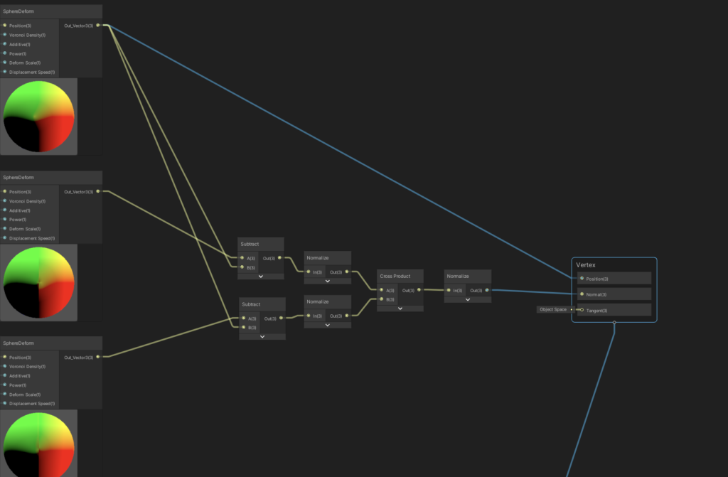
Finally, we’ll calculate two resultant vectors, normalize them, and then take the cross product. We then feed that into the “Normal” output of the shader.
Check out our sphere now in the scene view. It’s looking much better!
Our last step in this tutorial is to feed this material into a particle system, for dynamic-looking smoke. Unfortunately, our work is not done yet, as we’ll need a few adjustments to our shader to have it work on a per-particle basis.
Part 4 – Working with the Particle System
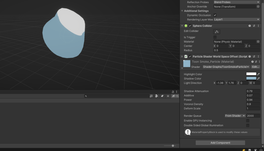
If we set up a Particle System right now, and applied our material to it, we’d end up with something that looked like this.
Some observations:
- The deformation is blowing up, causing each offset to blow past our clamped bounds (and thus giving each particle a perfectly spherical shape)
- As each particle moves, its deformation speed gets much faster (slightly hard to notice in this video)
To understand why each of these issues occur, we need to understand a little more about what happens to meshes when they’re fed into a Particle System.
For (very important) performance reasons, Unity batches each mesh in a Particle System into one combined mesh. There is a lot of technical detail in that process that I’m going to hand-wave away, but it has some practical implications that affect us. Particularly, each vertex within the Particle System gets transposed to World Space — within a particle system, we have no built-in way of accessing the object-local positions of a sphere’s vertices.
This means that, for each vertex that we process in our current shader:
- The offset we calculate will be the same unit magnitude for every sphere, no matter the sphere’s current size (“size” isn’t a concept in our shader currently — our only input is “position”)
- As each particle in the system moves, their vertices’s positions will change as well (as each vertex is translated into World Space)
Fortunately, Unity provides a facility named Particle Vertex Streams that allows us to input particle-specific data into our shader. We can solve our above problems by a) taking the “Size” parameter of each particle as input, and then normalizing our deformation offsets based off of that, and then b) transforming each vertex position into local space, using the particle’s “Center” parameter (alongside an additional World Position parameter that we’ll add to the overall material, via Material Property Block).
Lastly, we’ll input a random per-particle value and use it to offset our deformation. This will give each particle in the system some additional variation.
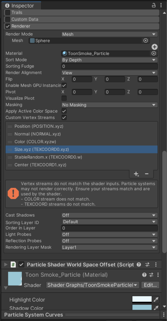
Enable the ‘Custom Vertex Streams” checkbox, remove the UV stream (we aren’t using it, so it’s just taking up extra space), and then add the Size, StableRandom, and Center vertex streams. Next to each vertex stream is the channel that it’s input to the shader as. For example, Size is input via the UV0 channel, via the x, y, and z segments of the vector.
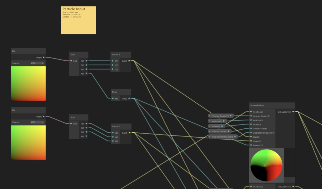
We’ll hook up the inputs inside of our graph now. Add “Size”, “Center”, and “Random” inputs into our deform sub-graph as well, and then make sure all of the wires are crossed correctly.
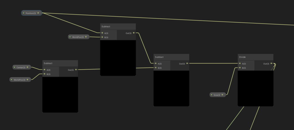
Additionally, we need to input the “World Position” of our Particle System GameObject into this shader. Our general strategy is to, for each particle, find the offset between the particle’s center and our system’s center, and then we’ll apply that offset to each of our particle’s vertices. This keeps each vertex to a local coordinate space, regardless of how it moves within the overall batched Particle System. Doing this is key to prevent the particle from deforming in unwanted ways as it moves through the world.
using UnityEngine;

[ExecuteInEditMode]
[RequireComponent(typeof(Renderer))]
public class ParticleShaderWorldSpaceOffset : MonoBehaviour
{
    Renderer _renderer;

    static readonly int WorldPos = Shader.PropertyToID("WorldPos");

    MaterialPropertyBlock _propBlock;

    void Awake() {
        _renderer = GetComponent<Renderer>();
        _propBlock = new MaterialPropertyBlock();
    }

    void Update() {
        _renderer.GetPropertyBlock(_propBlock);
        Vector3 existingWorldPos = _propBlock.GetVector(WorldPos);
        if (existingWorldPos != transform.position) {
            _propBlock.SetVector(WorldPos, transform.position);
            _renderer.SetPropertyBlock(_propBlock);
        }
    }
}
Add a “WorldPos” property to our shader (and to our deform sub-graph), and attach the following script to our Particle System. This will, every frame, update our shader with the World Position of our system, via Material Property Block.
In the deform sub-graph, our first step is to transform our input position into a local coordinate, and then to divide that position by our “size” input. This will give us a local, normalized position that we can feed into our noise.
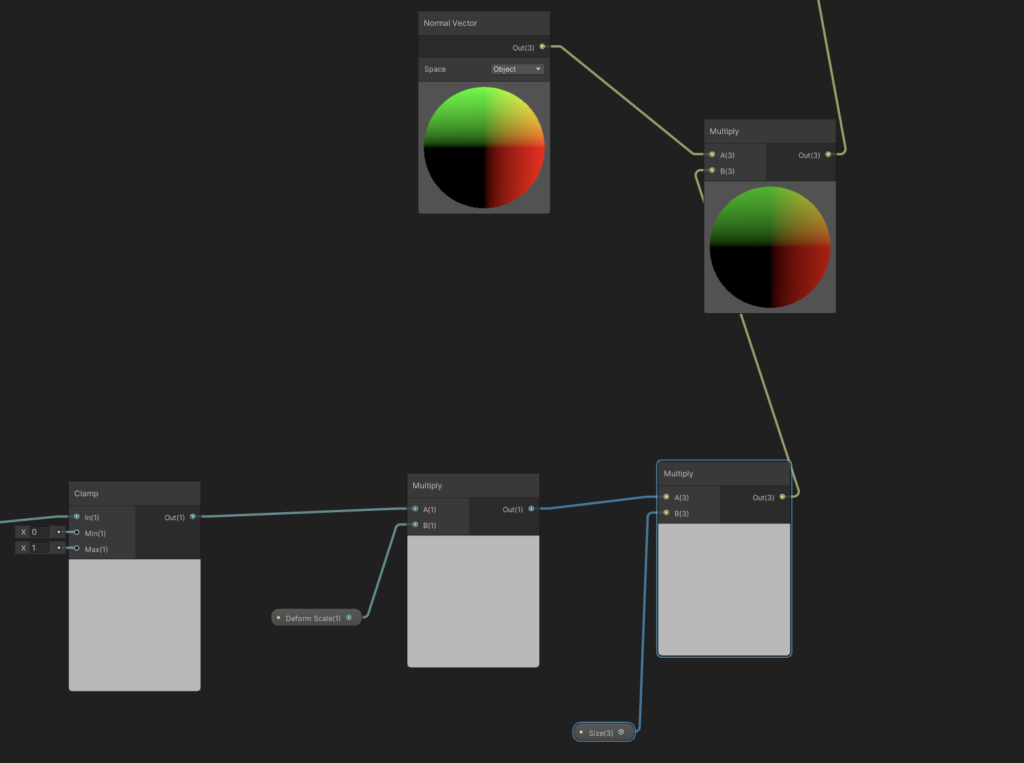
From there, the only other step is to, after calculating our offset, multiplying it back by our “Size” parameter, so that we’re offsetting by an amount that’s in-line with how big our sphere is.
Last step (and I mean it this time!), add a random range to our time offset, introducing a small amount of variability between the particles.
Let’s save our graph and check things out!
I think the smoke is looking pretty decent at this point. Things definitely converged a little late with our approach here, but we’ll finally shelve this one and call it done.
I’m attaching the Shader Graph for this smoke effect below. I hope you find it useful. Good luck!